LLM Architecture Explained: What’s Actually Inside a Large Language Model

You type a sentence, hit enter, and a machine writes back something coherent. It feels like there must be a sprawling, mysterious apparatus behind the curtain. There isn’t. The surprising truth about LLM architecture is that nearly every model you’ve heard of the GPT family, Llama, Claude, Gemini, Mistral is built from the same repeating building block, stacked dozens of times. Learn that one block and you understand the whole class of models.

Before we start, one clarification that trips people up: “LLM architecture” means two different things depending on who’s asking. There’s the model architecture the neural network itself (the transformer). And there’s the system architecture everything you bolt around a model to ship a product (retrieval, orchestration, guardrails, APIs). This post is about the first one: what’s inside the model. Once you understand that, the system stuff makes a lot more sense too.

The Short Answer

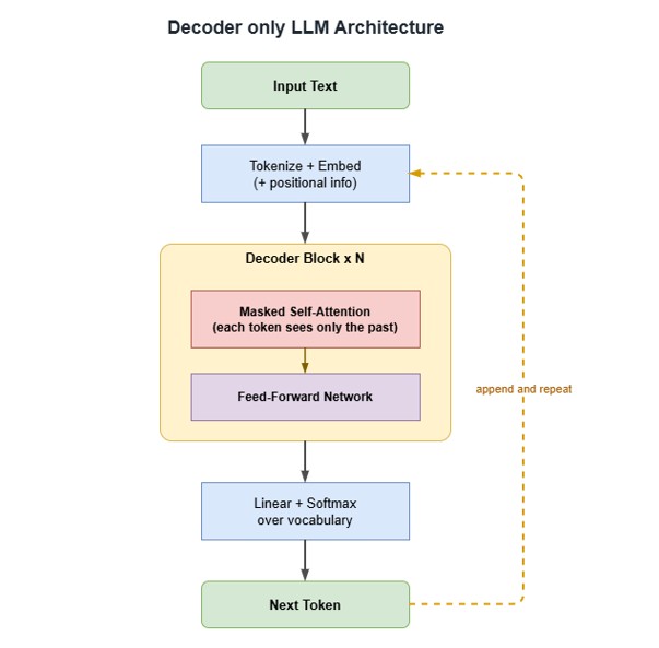
Modern LLMs are decoder-only transformers. Text is broken into tokens, each token becomes a vector (embedding), and those vectors flow through a stack of identical transformer blocks. Each block does two things: an attention step that lets every token look at the tokens before it, and a feed-forward step that transforms the result. After the final block, the model outputs a probability distribution over the next token. Generation is just doing this over and over, one token at a time. That’s it, the intelligence is an emergent property of a very large, very well-trained version of this simple loop.

Step 1: Text Becomes Numbers

A neural network can’t operate on characters, so the first job is turning text into numbers.
Tokenization splits your input into tokens usually subword chunks, not whole words. The word tokenization might become token + ization, while common words like the are a single token. Most models use a scheme like Byte-Pair Encoding (BPE) that balances vocabulary size against sequence length. A vocabulary of roughly 30,000 to 200,000 tokens is typical.

You can try GPT tokenzier here.

Each token maps to an ID, and each ID maps to a learned embedding a vector of, say, a few thousand numbers that encodes the token’s meaning. Embeddings are learned during training, so semantically related tokens end up near each other in vector space.

There’s one catch: attention (coming up next) has no inherent sense of order it treats a sequence like a bag of tokens. So we inject position information. Older models added fixed or learned positional encodings; most current models use Rotary Position Embeddings (RoPE), which encode position by rotating the query and key vectors. The practical upshot is the same: the model knows that “dog bites man” and “man bites dog” are different.

Step 2: Attention – The Core Idea

Self attention is the mechanism that made transformers work, and it’s the one piece worth understanding deeply.

For every token, the model computes three vectors by multiplying its embedding by learned weight matrices:

• Query (Q): what this token is looking for.
• Key (K): what this token offers to others.
• Value (V): the actual information this token passes along.

To decide how much token A should pay attention to token B, you take the dot product of A’s query with B’s key. High dot product means “relevant.” Those scores are scaled, passed through a softmax to turn them into weights that sum to 1, and used to build a weighted sum of the value vectors. In compact form:

Attention(Q, K, V) = softmax( (Q · Kᵀ) / √dₖ ) · V

That single equation is the heart of every LLM. It lets the word it in “the cup fell off the table and it broke” actually connect back to cup.

Two refinements make it powerful in practice:

• Multi-head attention. Instead of one attention calculation, the model runs several in parallel (each a “head”), each free to focus on a different kind of relationship grammar, coreference, topic. Their outputs are concatenated and mixed.
• Causal masking. In a decoder-only model, a token may only attend to tokens before it, never ahead. This is enforced by masking future positions with negative infinity before the softmax. It’s what makes the model able to generate text left to right without cheating.

A single attention head is one way of asking: “for each word, which other words should I look at?”

Why multiple heads

One head can only learn one kind of relationship. In “The cat that chased the mouse was hungry,” you need to know:

• was – agrees with cat (syntax)
• chased – links cat and mouse (who did what)
• hungry – describes cat (semantics)

One head averaging all of this gets mush. So you run h heads in parallel, each with its own small Q/K/V projections, each free to specialize. Then you concatenate their outputs and pass them through one final linear layer to mix them back into a single vector.

The trick: each head works in a smaller dimension, so 8 heads cost roughly the same as 1 big head. You get diversity for free.

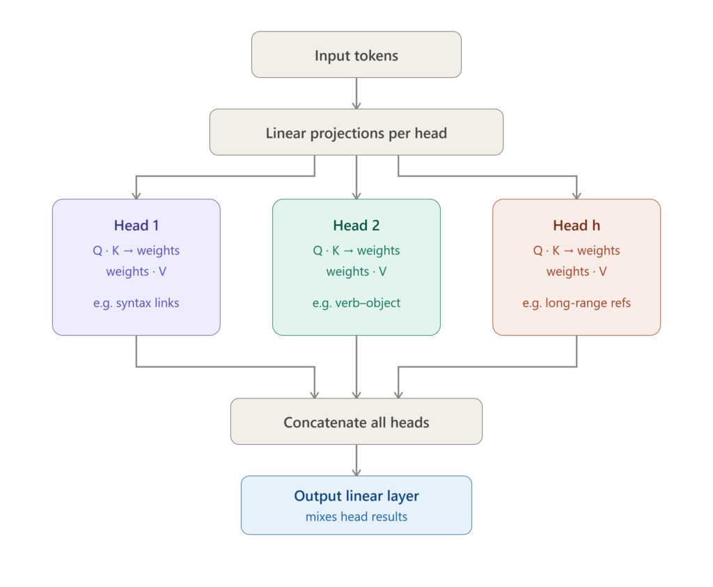
Quick analogy: a panel of h readers all read the same sentence. One tracks grammar, one tracks who-did-what-to-whom, one tracks pronoun references. Each writes a short note. An editor merges the notes into one summary. More readers with different specialties beats one reader trying to track everything at once.

Causal masking

Causal (autoregressive) masking stops a token from attending to anything that comes after it otherwise the model would cheat during training by peeking at the answer it’s supposed to predict.

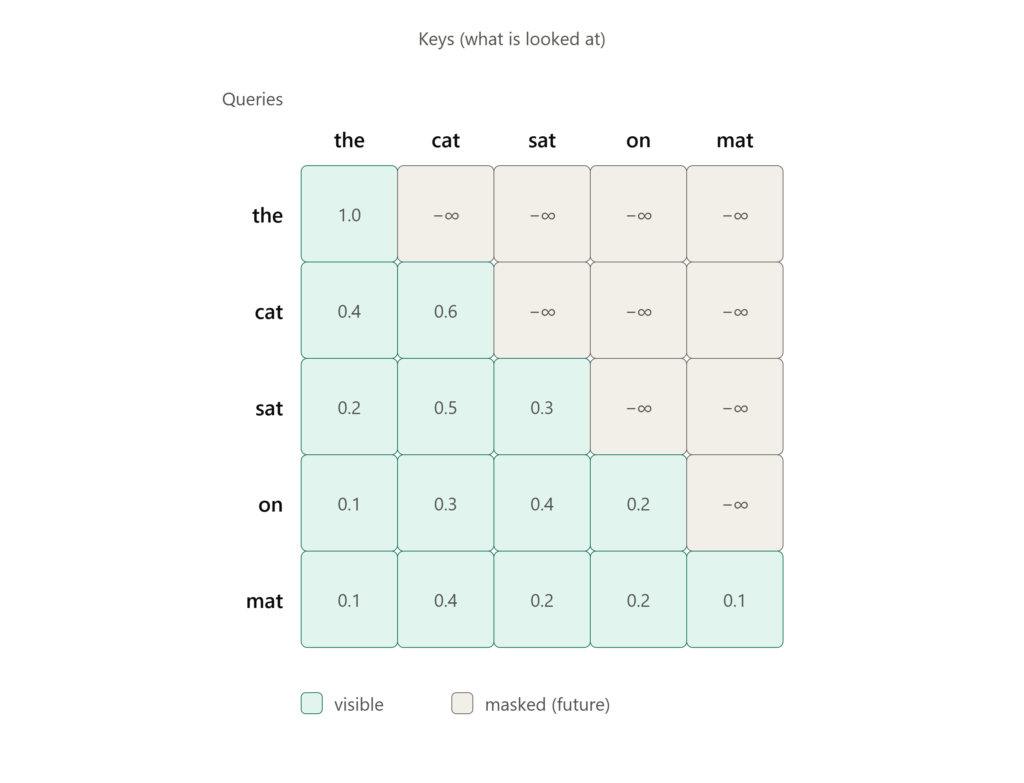
Each row is one token asking “who should I look at?” Row 1 (“the”) is the first word, so it can only see itself its weight is forced to 1.0. Row 5 (“mat”) is last, so it sees everything. The allowed region is a lower triangle, and each row’s surviving weights still sum to 1 after softmax.

Step 3: The Transformer Block

Attention is only half of each layer. A full transformer block wraps attention and a feed-forward network together with two features that make deep stacks trainable:

• A feed-forward network (MLP) – a small two-layer network applied to each token independently, usually expanding to ~4× the model width and back. This is where a lot of the model’s “knowledge” is stored.
• Residual connections – each sub-layer adds its output back to its input, giving gradients a clean path through dozens of layers.
• Normalization (LayerNorm or the increasingly common RMSNorm), typically applied before each sub-layer (“pre-norm”) for training stability.

import torch.nn as nn

class TransformerBlock(nn.Module):
    def __init__(self, d_model, n_heads):
        super().__init__()
        self.attn  = nn.MultiheadAttention(d_model, n_heads, batch_first=True)
        self.norm1 = nn.LayerNorm(d_model)
        self.norm2 = nn.LayerNorm(d_model)
        self.mlp   = nn.Sequential(
            nn.Linear(d_model, 4 * d_model),
            nn.GELU(),
            nn.Linear(4 * d_model, d_model),
        )

    def forward(self, x, causal_mask):
        # Pre-norm attention + residual
        h = self.norm1(x)
        attn_out, _ = self.attn(h, h, h, attn_mask=causal_mask)
        x = x + attn_out
        # Pre-norm feed-forward + residual
        h = self.norm2(x)
        x = x + self.mlp(h)
        return x

A real model just stacks this block N times 32, 80, sometimes more than 100 layers with the output of one feeding the input of the next. Model size (the “7B” or “70B” you see in names) is roughly the total parameters across all these blocks plus the embeddings.

After the final block, a last linear layer projects each position back to the size of the vocabulary. A softmax turns those numbers into probabilities, and the model has its prediction for the next token.

Step 4: Generation Is a Loop

To generate text, the model predicts a probability distribution for the next token, picks one (greedily, or by sampling with a temperature setting to control randomness), appends it to the input, and runs the whole thing again. This is why LLMs are called autoregressive: each new token is conditioned on everything generated so far.

A key optimization here is the KV cache. Because past tokens don’t change, the model caches their key and value vectors instead of recomputing them every step. This is why the first token of a response can feel slow (processing your whole prompt) while subsequent tokens stream quickly.

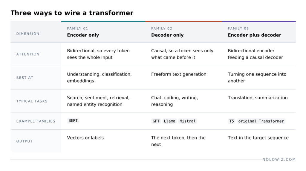
Not All Transformers Are the Same

Decoder-only is dominant today, but it’s one of three classic arrangements. Knowing the difference explains why BERT and GPT feel like different tools.

Which Architecture Should You Care About?

For most people building on LLMs today, the answer is decoder-only that’s what “LLM” almost always means now. But if you’re choosing a model type for a specific job, walk through these questions:

• Do you need to generate free-form text (chat, code, drafts)? Decoder-only. This covers the vast majority of modern use cases.
• Do you need to turn text into a fixed vector for search or classification? An encoder-only model (or a dedicated embedding model) is cheaper and often better than asking a generative LLM.
• Is your task a clean input to output transform like translation? Encoder-decoder can shine, though large decoder-only models now handle these tasks well via prompting.

Rule of thumb:

• Generating?  Decoder-only.
• Understanding or retrieving?  Encoder-only / embedding model.
• Faithful sequence-to-sequence transformation?  Encoder-decoder.
• Not sure? Default to a decoder-only model; it’s the most general.